Feb 21, 2019 | Munna K. & Patrick A.Before reading, you should watch the original video here. Special thanks to Scott Creager at Boulder AI. Step 0. Training vs. Test Data
Prior to covering facial detection and recognition, we need to specify the dataset we are working with.
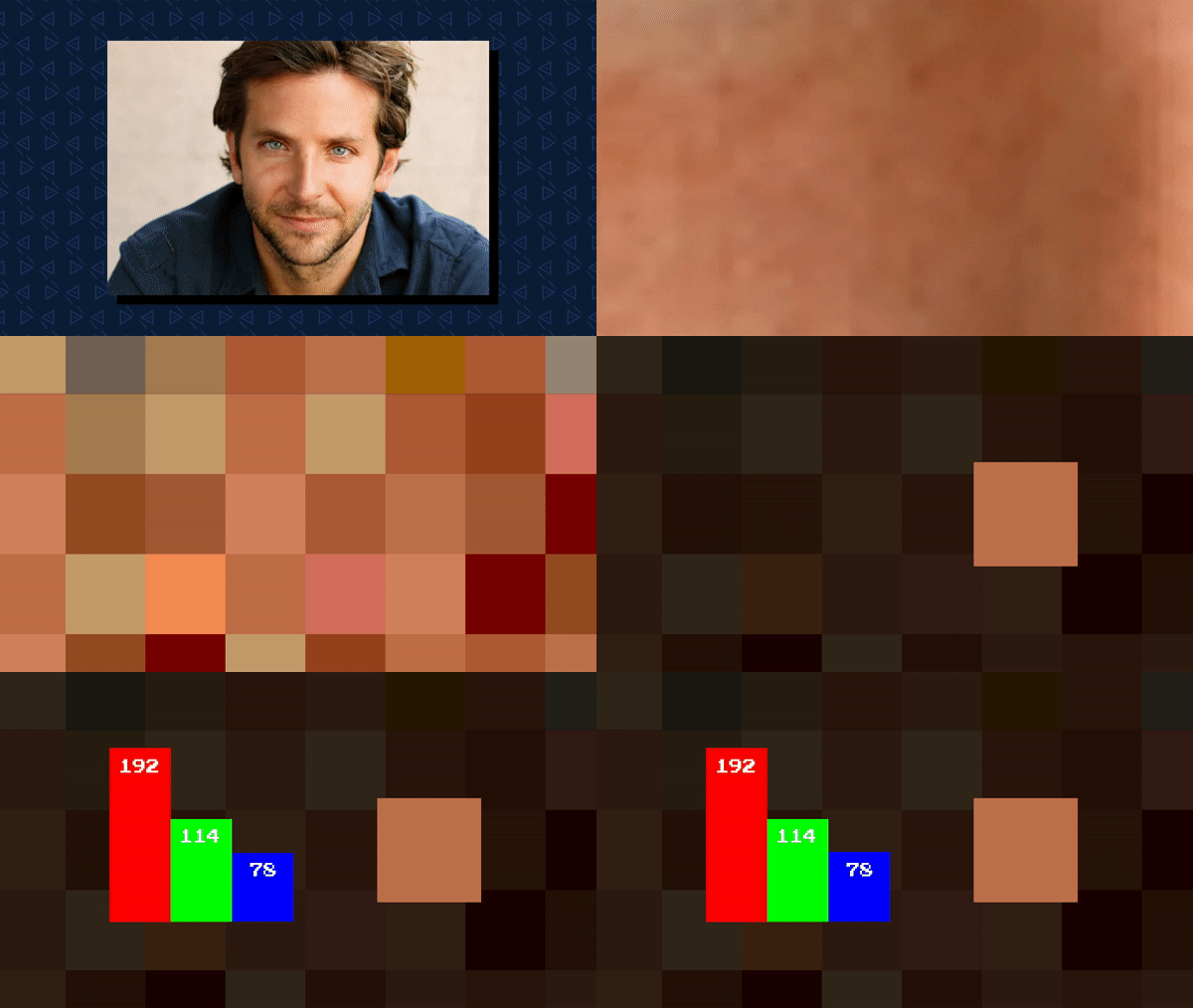
RGB Breakdown of an image of bradley cooper
How do algorithms “read” a picture? A picture is represented in computer vision algorithms as a matrix of pixels. Each pixel contains 3 values, one for each of the amount of red, blue, and green light at that pixel. For some aspects of facial detection, we instead use a single value for each pixel - the brightness intensity (see below).
brightness values of a picture of munna
The primary API we used, which you can find here, was trained on over 3 million images. The combined dataset was derived from the face scrub dataset, the VGG dataset, and a large number of images Davis King personally scraped from the internet. You can read more about the data on his post.
In machine learning models, training data is labeled: researchers know the image they are dealing with - and it has generally been validated by humans. Training pictures are used to help “inform” a computational model whether it’s correct in identifying a face, and typically include a lot of public pictures of known celebrities. For larger companies that have the access and tools, training data could also include your pictures (for example, if you share and tag your pictures on Facebook, Instagram, or Twitter).
typical breakdown of training data for machine learning models
How do you know a model is reliable and accurate? A portion of the dataset is set aside to test models (about 20%). A smaller portion of the dataset was used as “validation” data (about 16%), set aside for the purposes of fine-tuning parameters for the models that are used in face detection and recognition. Jason Brownlee has a great read about the training, validation, and test datasets here.
Step 1: Facial Detection (Training)
In the facial recognition process, the detection part is the most accurate and efficient. We are trying to answer two questions: Are faces present in the picture? If so, where are they?
To find any faces in the picture, we first scan the image for edges. Areas where brightness rapidly changes from one area to another represent what we see in the real world as edges. We then can tell the computer what patterns of edges make up a face. These include the oval container that we call a “face,” smaller circles that correspond to eyes, a mouth that runs across the face, etc. Edge detection is a common problem in the field of object detection, and the use of oriented gradients is a quick and easy solution.
showing the gradient at an individual pixel - this is before histogram calculation, which may alter the overall direction
For the video, we used the brightness values of an image to calculate the amount and the direction of change. To understand this, imagine seeing the grid of intensities like on the right, which shows the brightness values around a random, reference pixel (with brightness value 44). The edge in this case runs diagonally, from the upper-left to the lower-right. If we ask people to “point towards the brightest area,” relative to the center pixel, most would point towards the upper-right corner, perpendicular to the edge. To do this, our brain computes a “gradient” or directional change with respect to the reference pixel. The computer uses intensity, or brightness values around a pixel to do the same. We can compute the change for every pixel, and group the magnitudes by angles over a larger area, to compute the “histogram of oriented gradients” (HOG) for a block.
If you want more details on calculating gradients, Satya Mallick does a great explanation here.
The next step: finding the HOG patterns that match up to a face. The figure on the right is a typical HOG pattern of a face. The primary models used for face detection with HOG template matching are support vector machines (SVM). Basically, for each frame in a video, you can imagine a scrolling window, that outputs some probability that the object within it is a face, scrolls across a little, outputs the probability that the object within the new window is a face, and so on. The likelihood that the area within a window has a face is based on how closely the gradients within the window match the combination of gradients that make up a “typical” face.
Here is a great post that uses SVM and HOG models for detecting vehicles; this is a more technical explanation of SVM models in machine learning.
the sliding window detection method for facial detection - the hog for each window is compared with a reference face hog pattern to determine whether a face is detected
Step 2: Landmark Detection (Normalization)
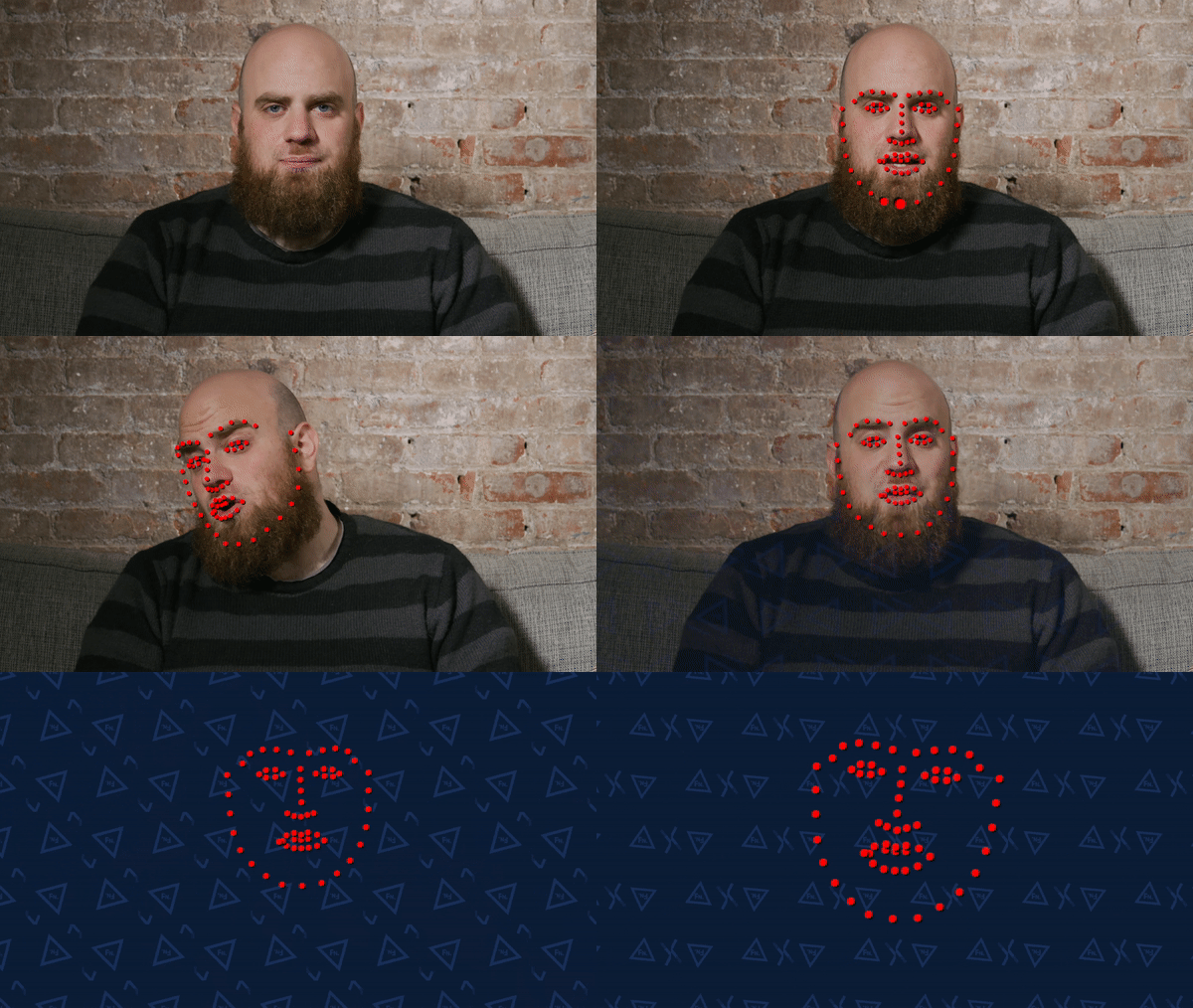
Landmarks are used in facial recognition to scale and align faces for more accurate comparisons.
Facial landmarks on patrick’s face - these are determined using iterative placements
The process for identifying landmarks involves first training a model using existing, human-coded data. The dataset that was used to train landmark data was HELEN, which you can read details about here. Thousands of people contributed by hand-marking data on over 2,000 images, placing landmarks that correspond to unique, defined points on the face shown in the figure on the left.
The specific algorithm that found landmarks on faces in our video was based on work by Vahid Kazemi and Josephine Sullivan, and involved initially estimating landmarks on a face, and then iteratively modifying them until the placement is correct. In the figure below, T labels the amount of times that the algorithm adjusted landmarks before contorting to the face.
So far we have glossed over how exactly you know you have the correct placement of landmarks. That is a relatively easy problem to solve and relies on a simple understanding: we know how the content behind landmarks relate to each other.
For example, we know that the color of our left eyebrow is constant throughout (unless you have a pretty crazy dye job). So if our initial placement of the landmarks yields different values for all “eyebrow landmarks,” then we know that the placement is probably not correct and we need to move it a bit to the left or right to get them correct. We loop through various placements, until the values for color and brightness behind each landmark match what we expect from a face (which we learned from our training dataset).
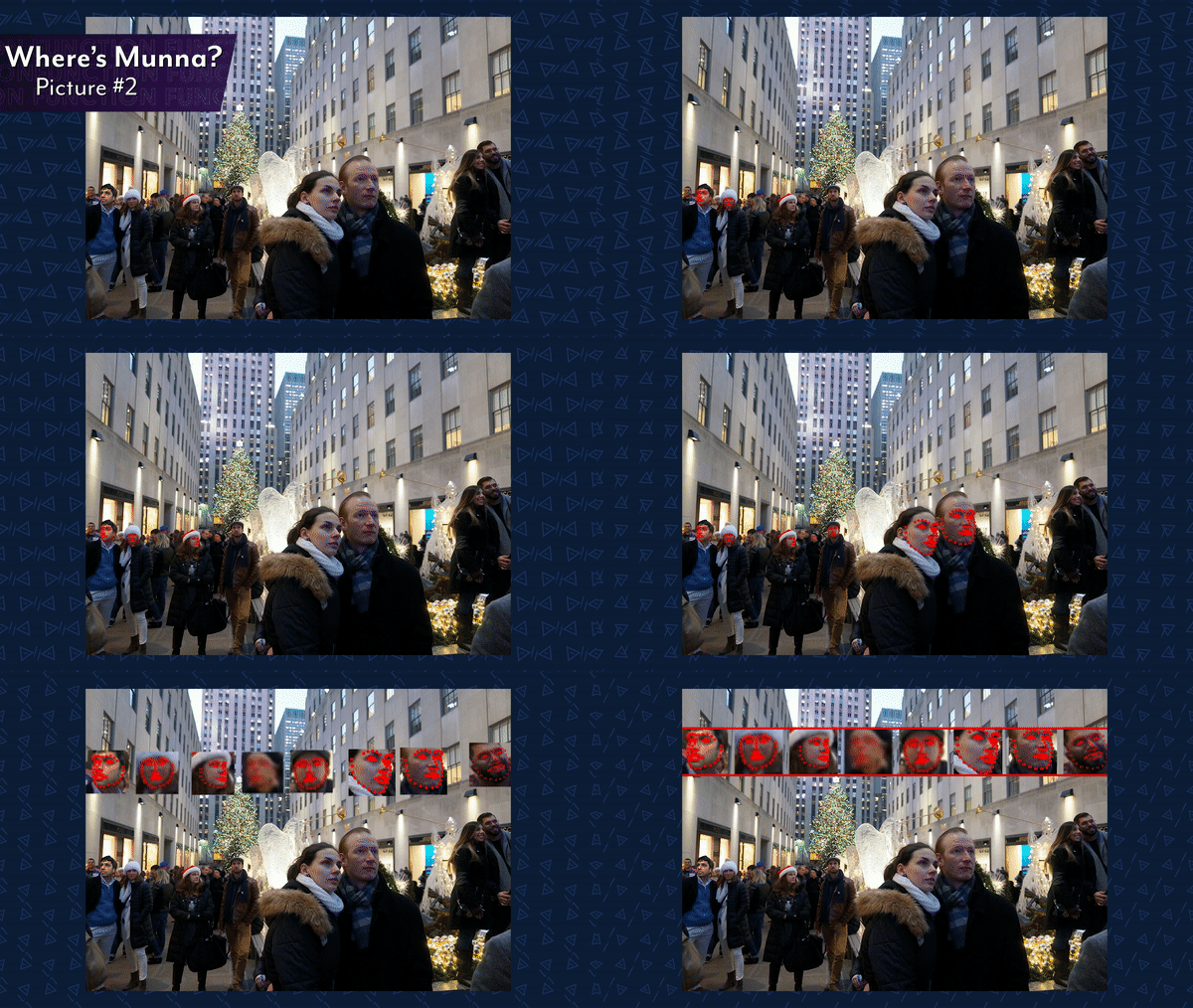
The goal of calculating landmarks is to allows us to normalize all faces. Before we can compare the faces in a complicated scene like below, we need to scale and rotate each face so that we can compare them. The placement of landmarks helps us orient the faces to be on the same relative axes.
landmark detection and normalization for a “Where’s Munna” picture
Step 3: Facial Recognition (Training)
This is the hard part. How can we distinguish between one person and 7.5 billion other people in this world? Deep learning models allow us to learn the complicated features that are required for a task like this.
a sample training dataset of a dreamy bradley cooper - celebrities are often used for training models
The next two sentences should sound familiar to you after reading the last sections. To train a facial recognition model, we work with a set of training data that is specific to each person. Unless you’re a truly unique looking person, one image is not enough to distinguish you from everyone else.
Before we get into the details, it’s helpful to understand the point of the training process. In the video, we present a 2-dimensional score that is unique to each person. In reality, this could be 64 or even a 1,000-dimensional score (the higher dimensions allow more freedom in finding differences between individuals). Most models, including ours, use 128-dimensional vector output. These embeddings, or output scores from the neural network, are used to compare images and people. For now, we will continue to simplify this so it’s easy to visualize on a 2-D grid. You can see that the embeddings for the training pictures of Bradley Cooper are close in distance to each other, while far away from pictures of other people.
a 2-dimensional face space showing placement of scores for various faces - Bradley’s scores are close together but far apart from the others (george takei, lady gaga, munna) the training process forces this result through adjusting weights
Our model compared outputs from three pictures at a time, two belonging to the same person and one belonging to another person. This is called triplet loss and is explained here. The two pictures belonging to a single person (e.g. Bradley Cooper) are labeled as “anchor” and “positive” examples in the figure below. An “antagonist” picture is one that belongs to another person (e.g. George Takei), and is labeled as a “negative” example below. After we process all three images, we can change the recognition model until the two pictures belonging to Bradley are close in their scores, and George’s scores are far away from both, known pictures of Bradley. If we do this for the large training dataset, for many different combinations, we know how to modify our model until it gives us an output where pictures of different people result in different scores. In this way, the model learns how to distinguish between features across thousands of people.
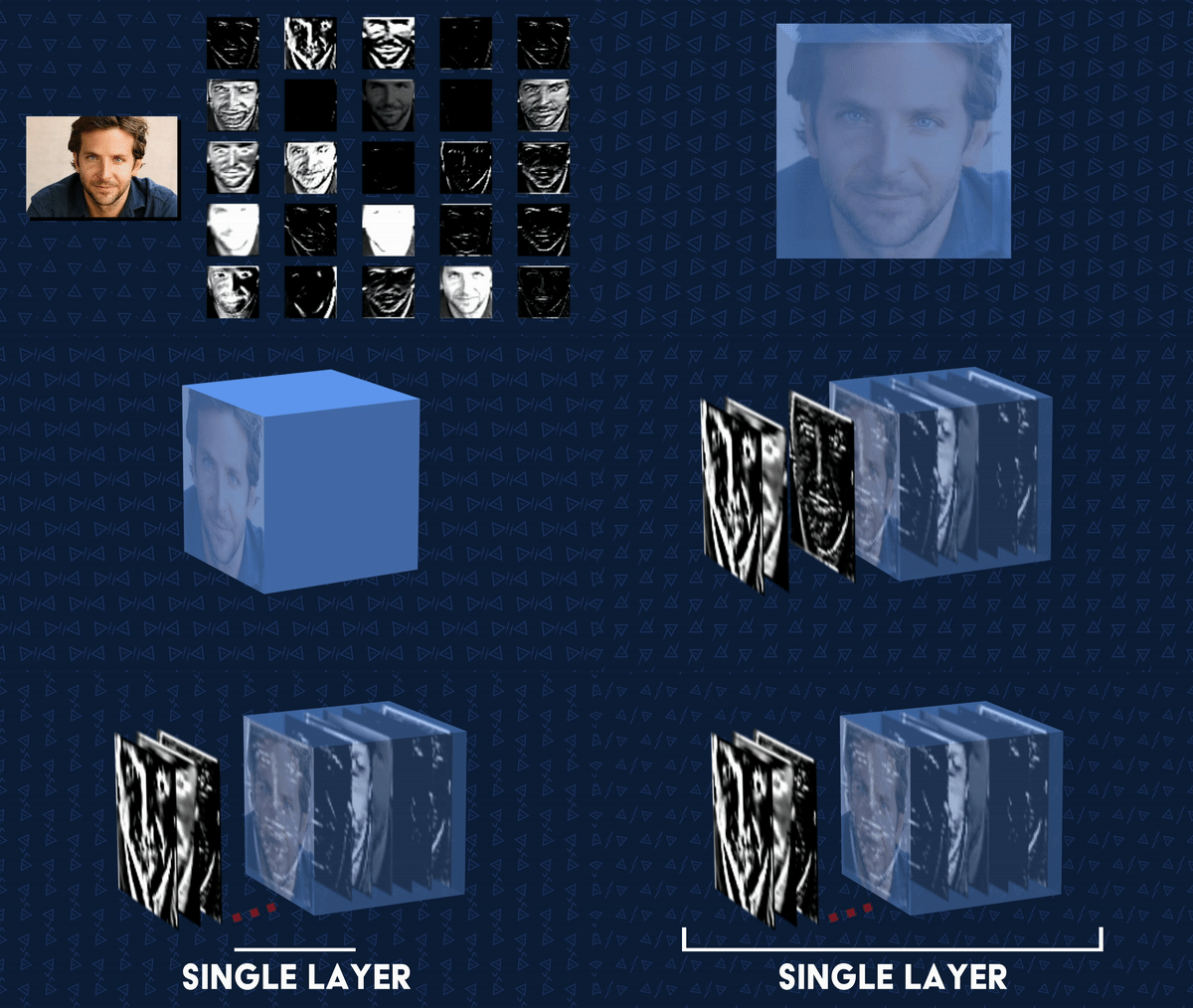
feature map generation using a simple edge filter on a picture of bradley cooper - in reality, these are harder to interpret
Now for the actual modeling, which uses a convolutional neural network (CNN). To understand the process, see the figure on the left showing what the first convolutional layer of the CNN is doing to the training image, which we show as a 3-D matrix of RGB layers (we’ve shown this before in in Step 0). The grey cube is a “kernel” or filter that convolves, or modifies the training image. It does this through “weights” or numbers that transform the input by multiplying and adding values. The modified image, or output, is what we refer to as a feature map, which is generated after the modifications. The edge filter that we show in the video (on the right) is the grey cube on the left, that runs through the entire training image to generate the convolution, or filtered output. The depth of a convolution layer, or the number of filters, can vary.
the first layer of a convolutional neural network - takes in a picture with RGB values to generate a large number of feature maps per layer
the pooling process reads each feature map and reduces the resolution by taking the max values in a moving window - it’s placed between conv layers
The filters within a single layer are independent (they don’t read each other) and are often reduced in size through a processed called “pooling.” We refer to the pooling process as average in the video for simplicity, but in facial recognition models the process uses max pooling, or finds the maximum value over a larger region. In the example on the right, the 4x4 matrix gets reduced to a 2x2 matrix. This loses some information in each filter, but is more efficient when we work with large data and has the added benefit of being robust, or resistant to minor variations in image (for example, hair covering a face).
The recognition network takes in a training image, which is then passed through a convolutional layer. Then, that layer is pooled, and passed through another convolutional layer. This process is repeated over and over again. The complexity of the filters increases, because the convolutional layers have a lot more data to mold, the further we get into the network. The final layer in the network is very large, and comprised of over 600 filters. All this information is reduced to a 128-dimensional score that is unique to each training image. These scores are compared to other training images, through a triplet comparison process (discussed above). The weights of the filters are then adjusted to so that all pictures of the same person (e.g. Bradley Cooper) have similar scores to each other but have different scores when compared to other people that do not look like Bradley Cooper. On the face map image we used, the pictures of Bradley Cooper are close together, and are far away on the grid from George Takei, who is himself far away on the grid from Munna. At this point, comparing pictures is as simple as comparing the Euclidean distance (the kind learned in high school geometry class) of scores. The entire training process is shown below.
a summary graphic of the facial recognition training process - from input to the final score generation for a training image after weight adjustments
If you are interested in more details about CNNs, we highly recommend Andrej Karapathy’s course on the topic, found here.
Step 4: Testing
After the training process, we have a model that understands the concept of a “face” very well. It contains filters that can “break down” a face into complicated representations, which we learned by providing the model with millions of faces in the training phase.
We can now input any picture, and get a score for each face found by the model. We can then compare this set of scores to scores for Bradley Cooper, George Takei, Lady Gaga, Patrick, Munna, etc. to see how close our test face is to a reference picture that we can also provide the model. Thus, a single run of our program required an input of two pictures: a “Where’s Munna” picture, and a reference picture of Munna. The process goes like this:
All the faces are detected in a “Where’s Munna” picture,
All the detected faces are normalized,
All the normalized faces are inputted into the CNN,
We receive an output (128-dimensional score) for each face that was detected and normalized,
We compare the scores for all the processed faces to Munna’s reference score, which we calculate separately.
If the scores for any of the faces are close enough to Munna’s reference score, then we found him. We designed the pictures so that Munna was always found by the computer (so we have something to compare to), and used MTurk to provide the same “Where’s Munna” pictures to humans for comparison.
You can see the results here: http://www.fractal.nyc/wheresmunna#data
If you have any questions or for more information, contact us at info@fractal.nyc.
